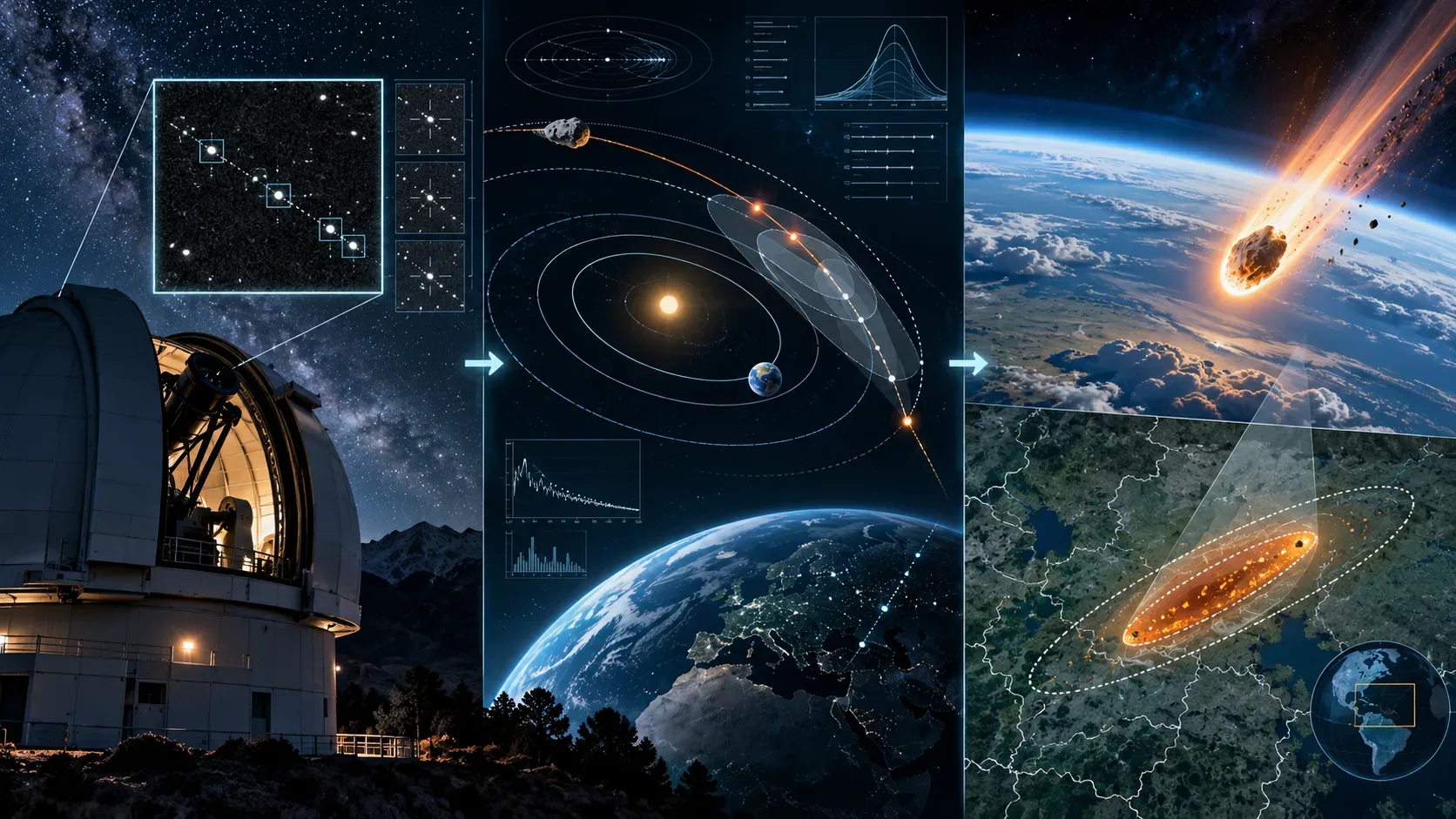
2026 RW1 highlighted an important difference between “seeing a fireball” and “predicting where it enters and where fragments could land.” In the case reported by ESA’s Near-Earth Object Coordination Centre (NEOCC), the prediction did not depend on direct footage of the atmospheric passage: it began with asteroid positions measured by telescopes, moved through orbit and entry-corridor refinement, and ended with a probabilistic simulation of atmospheric flight.
ESA says 2026 RW1 entered the atmosphere over the Indian Ocean, between Western Australia and the Lesser Sunda Islands, and was the 13th asteroid discovered on an impact trajectory. The interval from discovery to entry was only a few hours. Two official pages use different rounded figures: the NEOCC news item says “about 5 hours” before impact, while the event page says impact occurred “about 7 hours” after discovery. The safe conclusion is that the pipeline had to operate on a very short warning timescale.
What was estimated without direct footage
Without fireball-camera triangulation, NEOCC could still estimate two different things. The first was the entry state: where and how the object would reach the upper atmosphere. The second was the probabilistic strewn field: the region where surviving fragments would be more likely to reach the surface after ablation, fragmentation and dark flight.
Those predictions are not synonyms. The entry corridor comes mainly from the orbital solution. The strewn field requires atmospheric physics plus uncertainty about the body itself. ESA’s technical news item states that, for 2026 RW1, the derived uncertainty on the entry point was below 100 metres. That does not mean every surviving fragment would land inside a 100-metre circle: after entry, winds, drag, mass loss and successive breakups spread the possible ground locations.
1. Astrometry: turning points in the sky into a trajectory
The first link in the chain is astrometry. Each telescopic observation gives the object’s apparent position in the sky at a known time. A single position does not define an orbit; a sequence of measurements constrains the distances, directions and velocities compatible with the data.
For 2026 RW1, ESA’s event page says that after discovery by the Catalina Sky Survey’s Mt. Lemmon station, the asteroid was followed by three facilities in the US South-West and then by the Zadko and LCO Faulkes South telescopes in Australia, until the object entered Earth’s shadow. Two prediscovery positions from Pan-STARRS 2 were also reported. ESA says those added measurements refined the impact trajectory to sub-kilometre and sub-second levels.
The improvement comes from geometry: the more reliable positions are available and the better they are distributed in time, the smaller the region of orbits still compatible with the observations tends to become. NEOCC repeats the calculation as new astrometry arrives instead of treating the first solution as final.
2. Orbit and corridor: Meerkat flags, Aegis refines
In ESA’s operational chain, Meerkat monitors candidates for imminent impact and rapidly evaluates possible trajectories. When an object reaches a significant impact probability, Aegis takes over orbit refinement, computes the solution covariance and produces the impact corridor.
The paper describing the new method gives an operational trigger: with more than four observations and an impact score above 10%, Aegis refines the orbit; when impact probability reaches 100% and the 1-sigma uncertainty is below 10 km, the corridor can be passed to the strewn-field module. The system provides 1-, 3- and 5-sigma confidence contours for variables including latitude, longitude, velocity, flight-path angle and heading.
This is where “orbit” becomes “entry.” ESA uses the predicted state at 100 km altitude as the initial condition for atmospheric modelling. Up to that point, the calculation is asking where and with what velocity/direction the object crosses the upper atmosphere; it is not yet a meteorite-on-the-ground forecast.
3. From entry to ground: drag, ablation, fragmentation and dark flight
From 100 km downward, the problem changes. The model numerically propagates the object through the atmosphere, simulating aerodynamic drag, ablation — mass loss caused by heating — and a statistically defined cascading fragmentation process. Fragments created at each breakup are then tracked independently.
When a fragment has slowed enough to leave the luminous phase, it enters dark flight. At that stage, the fall is strongly affected by winds. The system uses atmospheric conditions and forecasts from the Global Forecast System (GFS) to propagate each fragment to the surface.
This design explains why the tool can work without a camera following the fireball. Direct footage would normally add valuable constraints on the real trajectory and breakup history, but the new method starts from the pre-impact orbit and plausible physical distributions to simulate many possible outcomes. ESA presents it as a complement, not a universal replacement, for camera networks.
4. Why the result is a probability, not an exact point
The main mechanism for handling uncertainty is a Monte Carlo method. Instead of choosing one value for everything that is unknown, the program repeats the simulation while varying the entry state, the body’s physical properties, fragmentation parameters and atmospheric conditions within assumed distributions.
The output is a two-dimensional probability map. In the work by Moscati and colleagues, successive simulations are aggregated until the map stabilizes according to a convergence criterion; the described operational upper limit is 1,000 runs, with convergence usually reached earlier.
This changes how the map should be read: the highlighted area does not mean “all meteorites will be here.” It shows where the set of simulated scenarios concentrates probability. Contours such as 50%, 80% or 99% represent cumulative portions of the predicted distribution, not physical fences on the ground.
5. A strewn field is not the same as recovered meteorites
A strewn field is a spatial prediction. Recovered meteorites are physical evidence found afterward. The distinction matters because a prediction can exist even when no fragment is recoverable, when the area is over the ocean, when fragments are too small, or when no search is conducted.
ESA illustrates this distinction with 2023 CX1: the pre-impact map shows probability curves, while overlaid crosses indicate meteorites that were actually recovered. A recovery falling inside a high-probability zone helps evaluate the model, but the absence of a recovery does not, by itself, prove that the map was wrong.
For 2026 RW1, atmospheric entry occurred over the Indian Ocean. The event is therefore especially useful for demonstrating the calculation chain without depending on a land-based recovery campaign: it is possible to estimate a fragment-fall region even when physical confirmation by recovery is impractical.
6. What uncertainty really means for 2026 RW1
There are at least three layers of uncertainty. The first is orbital: positions and times measured by observatories contain errors and leave a family of possible orbits. The second is physical: the mass, density, strength and fragmentation behaviour of a small asteroid are not perfectly known before entry. The third is atmospheric: winds and air density vary with altitude, location and time.
New observations mainly reduce the first layer. That is why NEOCC reruns the solution as data arrive and says the corridor and strewn field become more precise. The other layers do not disappear; they are exactly why the final result remains probabilistic.
The pipeline in practical terms
- Telescopes measure positions and timestamps for the asteroid.
- Meerkat rapidly evaluates whether compatible solutions point to impact.
- Aegis refines the orbit and corridor with new astrometry and covariance analysis.
- The state at 100 km altitude becomes the initial condition for atmospheric entry.
- Monte Carlo simulates many entries, varying body properties and uncertainties.
- Drag, ablation and fragmentation determine which fragments may survive.
- GFS winds drive dark flight down to the surface.
- The simulated impacts form a probability map, which can be updated as new observations shrink the orbital corridor.
What the case teaches about planetary defence
The value of the 2026 RW1 case is not a claim that every fragment can be located with absolute certainty. It shows that telescopic observations obtained only hours before entry can already feed an automated chain from astrometry to orbit, from orbit to entry state, and finally to a probabilistic strewn field.
That is useful in two settings. For small objects, it can guide rapid searches for freshly fallen meteorites and reduce terrestrial contamination of samples. For larger objects, the same logic can support situational assessment by planetary-defence and civil-protection teams — but the paper itself stresses that decisions such as evacuation or infrastructure closure require other layers, including exposed population, land use and vulnerability.
Main sources: NEOCC/ESA: Predicting the strewn field of imminent impactors; NEOCC/ESA: 2026 RW1 event page; Moscati et al. (2026), Icarus: From orbit to ground.