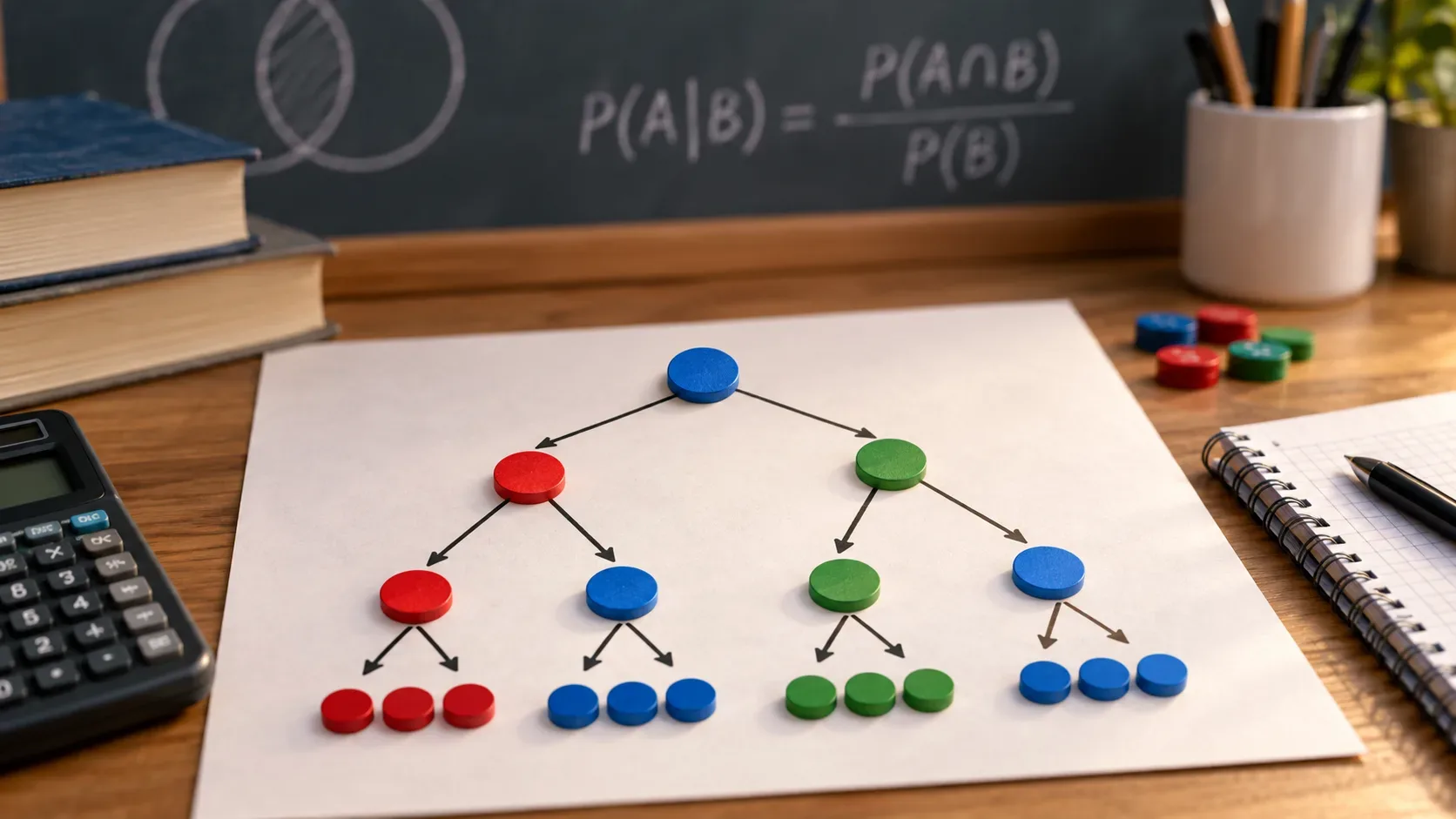
In a probability tree, the right operation depends on where you are looking: multiply along a path, add alternative terminal paths, and when a condition removes part of the tree, renormalize only what remains. This way of reading the diagram avoids memorizing isolated formulas and turns conditional probability into a visual procedure.
The method in one sentence
- Multiply here: when the question requires several stages on the same path to occur together.
- Add here: when the desired event can occur through different, mutually exclusive terminal paths.
- Renormalize here: when you learn new information, discard incompatible paths, and make the remaining total equal 1 again.
The idea follows the multiplication rule for multistage events presented by OpenStax and the interpretation of conditional probability as restricting the sample space described in UC Berkeley statistics material.
Base problem: which line produced a reviewed item?
A company receives 60% of its items from line A and 40% from line B. On line A, 10% of items are flagged for review. On line B, 20% are flagged for review. One item is chosen at random and we know it was flagged for review. What is the probability that it came from line B?
The tree starts with two source choices:
- Line A: 0.60.
- Line B: 0.40.
Then each source splits into “review” and “no review”:
- If it came from A: review 0.10; no review 0.90.
- If it came from B: review 0.20; no review 0.80.
1. Multiply here: calculate each complete path
Reaching a leaf in the tree means passing through a sequence of events. Therefore, the probability of each leaf is the product of the probabilities written on the branches along that path.
| Path | Calculation | Probability |
|---|---|---|
| A and review | 0.60 × 0.10 | 0.06 |
| A and no review | 0.60 × 0.90 | 0.54 |
| B and review | 0.40 × 0.20 | 0.08 |
| B and no review | 0.40 × 0.80 | 0.32 |
This is the multiplication-rule logic: to arrive at “B and review,” the item must first be in B and then follow the “review” branch. Thus, P(B and review) = P(B) × P(review | B) = 0.40 × 0.20 = 0.08.
2. Add here: combine paths that produce the same event
Now we want the total probability that an item is flagged for review, without yet conditioning on its source. “Review” can happen through two different terminal paths: A and review, or B and review. Because one item cannot simultaneously come from both lines, these leaves are mutually exclusive and can be added directly.
P(review) = 0.06 + 0.08 = 0.14.
This 0.14 matters: it is the entire probability mass that survives once we learn that the item was reviewed.
3. Renormalize here: make the condition the new universe
After receiving the information “the item was flagged for review,” the paths “A and no review” and “B and no review” are no longer possible. Only 0.06 from A and review and 0.08 from B and review remain. Together they sum to 0.14, but inside the new conditioned universe that total must represent 1.
Renormalizing means dividing each surviving path by the surviving total:
- P(A | review) = 0.06 ÷ 0.14 ≈ 0.4286, or 42.86%.
- P(B | review) = 0.08 ÷ 0.14 ≈ 0.5714, or 57.14%.
Therefore, once we know the item was reviewed, line B becomes the more likely source even though it produces only 40% of all items. That is because the review rate is higher on B. The operation “divide by the total that survived” is exactly the logic of P(A | B) = P(A and B) / P(B): the condition redefines the relevant sample space.
4. Final verification
Before finishing, run four simple checks:
- The branches leaving each node sum to 1: 0.10 + 0.90 = 1 and 0.20 + 0.80 = 1.
- The four leaves sum to 1: 0.06 + 0.54 + 0.08 + 0.32 = 1.
- The total probability of the conditioning event is between 0 and 1: P(review) = 0.14.
- After renormalization, the conditional alternatives sum to 1: 0.4286 + 0.5714 = 1, up to rounding.
How to choose between multiplying, adding, and renormalizing
| Signal in the question | Operation | What you calculate | Example |
|---|---|---|---|
| “and then,” “and,” a sequence of stages | Multiply | Probability of one complete path | A and review: 0.60 × 0.10 |
| “or,” “through any of these paths” | Add leaves compatible with the event | Total probability of an event with alternative routes | Review: 0.06 + 0.08 |
| “given that,” “knowing that,” “among those who...” | Renormalize | Probabilities inside the new conditioned universe | B given review: 0.08 ÷ 0.14 |
Why adding leaves is usually simple
The general rule for “A or B” is not always simple addition. When two events can occur at the same time, their intersection must be subtracted. But different terminal leaves of a probability tree represent mutually exclusive outcomes: an experiment ends at one leaf or another, not both. Therefore, when you combine terminal leaves that satisfy the event of interest, direct addition is valid. OpenStax uses this same property when adding final outcomes in tree diagrams.
Independence changes the numbers, not the method
If the second stage is independent of the first, the probability on the second branch does not change with the first result. In that case, P(B | A) = P(B), and the path product can be written as P(A) × P(B). But do not use that form automatically. In conditional-probability problems, it is safer to ask first: “does the probability of the next branch depend on what has already happened?” If it does, use the conditional probability shown at that node.
Renormalizing is Bayes viewed through the tree
Many problems ask for the reverse direction of the information given. In the example, we know P(review | A) and P(review | B), but the question asks for P(B | review). The tree solves this reversal without requiring you to start from Bayes’ formula: first multiply to get the complete paths, then add to find the probability of the evidence, and finally divide the path of interest by that total. The compact Bayes formula is one way of writing these same three steps.
Common mistakes the tree helps prevent
- Adding probabilities on consecutive branches. Branches on the same route form a sequence; a path is calculated by multiplication.
- Multiplying alternative paths. If the event can happen through one leaf or another, combine those leaves by addition.
- Using 20% as the final answer. The 20% is P(review | B), not P(B | review). Reversing the condition changes the question.
- Renormalizing before calculating the leaves. First determine how much each path contributes to the observed event; only then divide by the observed total.
- Forgetting to check the total. A complete tree should end with leaves that sum to 1, apart from rounding.
A procedure that works on exercises
- Identify the stages and draw a node for each decision point.
- Write a valid probability on each branch for that node; branches leaving the same node must sum to 1.
- Multiply along each path to obtain the leaf probabilities.
- Mark which leaves satisfy the event being asked about.
- Add those leaves if there is more than one possible path.
- If the question contains “given that” or provides new information, discard incompatible leaves and divide each survivor by the sum of the survivors.
- Run the final check: totals between 0 and 1 and, where appropriate, sums equal to 1.
The main point is operational: the shape of the tree tells you which calculation to perform. A complete path calls for multiplication; alternative terminal paths call for addition; new information calls for restriction and renormalization. With that map, formulas stop being disconnected rules and become compact summaries of reasoning you can already see.